SQL Pattern Matching Deep Dive - Part 2, using MATCH_NUMBER() and CLASSIFIER()

Welcome to the second post in this deep dive series on SQL pattern matching using the new MATCH_RECOGNIZE feature that is part of Database 12c. In the first part of this series we looked at the areas of ensuring query consistency, how to correctly use predicates and how to manage sorting.

In this post I am going to review the two built-in measures that we have provided to help you understand how your data set is mapped to the pattern that you have defined. This post will breakdown into three areas: 1) a review of the built-in measures, 2) understanding how to control the output (number of rows returned) and lastly I will bring these two topics together with some examples.

 

Built-in measures

We provide two built-in measures to help you understand how your data maps to a pattern: MATCH_NUMBER() and CLASSIFER(). These two functions are typically included as part of the MEASURE clause. It is possible to use them within other areas of the MATCH_RECOGNIZE clause but, in many cases, they are of limited use because in the majority of cases the information returned would not make a lot sense or have very very limited meaning.

To get you started here is a quick definition of each function:

MATCH_NUMBER()

You might have a large number of matches for your pattern inside a given row partition. How do you tell these matches apart? This is done with the MATCH_NUMBER() function. Matches within a row pattern partition are numbered sequentially starting with 1 in the order they are found. This numbering starts at 1 within each row pattern partition, because there is no linked ordering across row pattern partitions.

CLASSIFIER()

Along with knowing which MATCH_NUMBER you are seeing, you may want to know which component of a pattern applies to a specific row. This is done using the CLASSIFIER() function. The classifier of a row is the pattern variable that the row is mapped to by a row pattern match. The CLASSIFIER() function returns a character string whose value is the name of the pattern variable defined within the PATTERN clause.

These two functions will typically only be used within the MEASURE clause. Interestingly, it is possible to use both these functions within the DEFINE clause but it is doubtful, at least in my mind, as to whether this would ever be useful. However, the following is possible:

DEFINE X AS (MATCH_NUMBER() <= PREV(price)),
Y AS (price >= PREV(price)),
W AS (price <= PREV(price)),
Z AS (price >= PREV(price)));

or you could have:

DEFINE X AS (CLASSIFIER() <= ‘Z’),
Y AS (price >= PREV(price)), 
W AS (price <= PREV(price)),
Z AS (price >= PREV(price)));

The SQL code will compile and execute but is it useful? Let me know if you can find a use case for putting these functions within the DEFINE clause.

Controlling the output

The return values from both the above functions is determined by the type of output defined as part of the MATCH_RECOGNIZE clause. Sometimes you want summary data about the matches within your data set and other times you need the full details. You can do that with the following syntax:

ONE ROW PER MATCH : each match produces one summary row. This is the default output.

ALL ROWS PER MATCH : a match spanning multiple rows will produce one output row for each row in the match. There are three sub options:

• ALL ROWS PER MATCH SHOW EMPTY MATCHES - note this is the default
• ALL ROWS PER MATCH OMIT EMPTY MATCHES
• ALL ROWS PER MATCH WITH UNMATCHED ROWS

The idea of having unmatched rows is largely self-explanatory or at least I hope that it is! The idea of having empty matches might take a little more thinking….Let’s look at a very simple pattern which permits empty matches: the pattern PATTERN (A*). This can be matched by zero or more rows that are mapped to A (this is what the identifier * implies).

An empty match does not map any rows to pattern variables but it does in fact have a starting row. For example, there can be an empty match at the first row of a partition, an empty match at the second row of a partition, and so on. An empty match is actually assigned a sequential match number, based on its position with respect to the starting row in just the same way as any other match.

If we are using the ALL ROWS PER MATCH syntax then we need to cater for two scenarios in relation to handling empty matches:

• ALL ROWS PER MATCH SHOW EMPTY MATCHES: with this option, any empty match generates a single row in the row pattern output table.
• ALL ROWS PER MATCH OMIT EMPTY MATCHES: with this option, an empty match is omitted from the row pattern output table. However, it should be noted that this may cause gaps in the sequential match numbering.

Using the ALL ROWS PER MATCH (which defaults to SHOW EMPTY MATCHES), an empty match generates one row in the row pattern output table where the measures will have the following values:

• CLASSIFIER() function returns null
• MATCH_NUMBER () function returns the sequential match number of the empty match
• value of any ordinary row pattern column reference is null
• value of any aggregate or row pattern navigation operation is computed using an empty set of rows (so any COUNT is 0, and all other aggregates and row pattern navigation operations are null).
• value of any column corresponding to a column of the row pattern input table is the same as the corresponding column in the starting row of the empty match.

 

Bringing it all together

First let’s start by using our normal stock ticker data set and searching for W-shaped patterns. Here is the code:

SELECT symbol, tstamp, price, first_x, last_z
FROM ticker
MATCH_RECOGNIZE (
  PARTITION BY symbol ORDER BY tstamp
  MEASURES FIRST(x.tstamp) AS first_x,
           LAST(z.tstamp) AS last_z
  ALL ROWS PER MATCH
  PATTERN (X+ Y+ W+ Z+)
  DEFINE X AS (price <= PREV(price)),
         Y AS (price >= PREV(price)),
         W AS (price <= PREV(price)),
         Z AS (price >= PREV(price)))
WHERE symbol='OSCORP';

…which returns the following output:

For the symbol OSCORP we have matched two W-shapes: the first starts on 02-APR-11 and ends on 08-APR-11 and the second starts on 09-APR-11 and ends on 16-APR-11. Now let’s introduce our built-in measures and see how our data set is being matched to our pattern. To do this we add the built-in functions to our MEASURE clause as shown here:

SELECT symbol,
  tstamp,
  price,
  match_number,
  classifier,
  first_x,
  last_z
FROM ticker
MATCH_RECOGNIZE (
  PARTITION BY symbol ORDER BY tstamp
  MEASURES FIRST(x.tstamp) AS first_x,
           LAST(z.tstamp) AS last_z,
           MATCH_NUMBER() AS match_number,
           CLASSIFIER() AS classifier
  ALL ROWS PER MATCH
  PATTERN (X+ Y+ W+ Z+)
  DEFINE X AS (price <= PREV(price)),
         Y AS (price >= PREV(price)),
         W AS (price <= PREV(price)),
         Z AS (price >= PREV(price)));

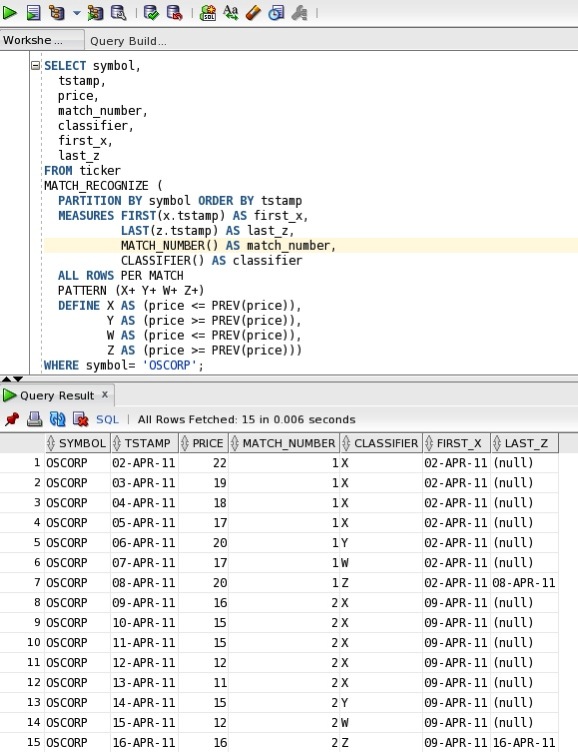
…which returns the following output:

 

Note that I have removed the WHERE clause so that you can see the how the MATCH_NUMBER() sequencing is handled across partition boundaries - i.e. you should note that the match numbering starts at 1 within each symbol-based partition. For symbol ‘ACME’ we have one matched one W-shaped pattern and the same applies to ‘GLOBEX’.

Within the OSCORP partition we matched two W-shapes. 

 If we change the output to included the unmatched rows it becomes a lot easier to check the pattern against the whole data set:

SELECT symbol, 
  tstamp,
  price, 
  match_number,
  classifier,
  first_x, 
  last_z 
FROM ticker
MATCH_RECOGNIZE (
  PARTITION BY symbol ORDER BY tstamp
  MEASURES FIRST(x.tstamp) AS first_x,
           LAST(z.tstamp) AS last_z,
           MATCH_NUMBER() AS match_number,
           CLASSIFIER() AS classifier
  ALL ROWS PER MATCH WITH UNMATCHED ROWS
  PATTERN (X+ Y+ W+ Z+)
  DEFINE X AS (price <= PREV(price)),
         Y AS (price >= PREV(price)), 
         W AS (price <= PREV(price)),
         Z AS (price >= PREV(price)));

…which returns the following output:

 

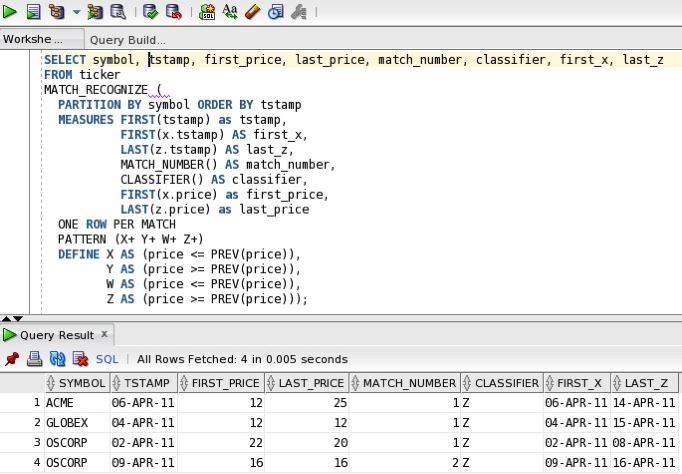
What happens if we switch to returning summary information:

SELECT symbol,
  tstamp,
  first_price,
  last_price,
  match_number,
  classifier,
  first_x,
  last_z
FROM ticker
MATCH_RECOGNIZE (
  PARTITION BY symbol ORDER BY tstamp
  MEASURES FIRST(tstamp) as tstamp,
           FIRST(x.tstamp) AS first_x,
           LAST(z.tstamp) AS last_z,
           MATCH_NUMBER() AS match_number,
           CLASSIFIER() AS classifier,
           FIRST(x.price) as first_price,
           LAST(z.price) as last_price
  ONE ROW PER MATCH
  PATTERN (X+ Y+ W+ Z+)
  DEFINE X AS (price <= PREV(price)),
         Y AS (price >= PREV(price)),
         W AS (price <= PREV(price)),
         Z AS (price >= PREV(price)));

 

…which returns the following output:

You should notice that the value returned by the CLASSIFIER() function is now truncated to the last variable listed in the DEFINE clause, which in this case is the pattern variable “Z”.  Therefore, when using CLASSIFIER() function to check how the pattern is being applied you should use one of the ALL ROWS PER MATCH options which allows you to see which rows are assigned to which pattern variable. The real benefit of this will become obvious when we look at greedy vs. reluctant quantifiers, which is coming up in a future post.

Note that even with the ONE ROW PER MATCH syntax the MATCH_NUMBER() function continues to operate as before. 

 

Summary

In this post we have looked at how to use the two built-in measures MATCH_NUMBER() and CLASSIFIER() within the MEASURES clause.  You can also use them in the DEFINE clause as well - if needed.

We have explored how the output from these measures changes as we switch from returning summary rows compared to detailed rows: ALL ROWS PER MATCH vs. ONE ROW PER MATCH. In the next post I will explore the concept of reluctant vs. greedy quantifiers.

Feel free to contact me if you have an interesting use cases for SQL pattern matching or if you just want some more information. Always happy to help. My email address is keith.laker@oracle.com.

 

Technorati Tags: Analytics, Database 12c, Pattern Matching, SQL Analytics